Pi Controller Phase Rises Again Before Falling
 |  |  |  | |
|---|
A variation of Proportional Integral Derivative (PID) control is to use only the proportional and integral terms every bit PI command. The PI controller is the near popular variation, even more than than total PID controllers. The value of the controller output `u(t)` is fed into the system as the manipulated variable input.
$$due east(t) = SP-PV$$
$$u(t) = u_{bias} + K_c \, eastward(t) + \frac{K_c}{\tau_I}\int_0^t e(t)dt$$
The `u_{bias}` term is a constant that is typically set to the value of `u(t)` when the controller is offset switched from transmission to automated mode. This gives "bumpless" transfer if the error is zero when the controller is turned on. The two tuning values for a PI controller are the controller proceeds, `K_c` and the integral time constant `\tau_I`. The value of `K_c` is a multiplier on the proportional error and integral term and a higher value makes the controller more aggressive at responding to errors abroad from the ready point. The set up point (SP) is the target value and process variable (PV) is the measured value that may deviate from the desired value. The error from the set up betoken is the divergence between the SP and PV and is divers as `e(t) = SP - PV`.
Detached PI Controller
Digital controllers are implemented with discrete sampling periods and a discrete form of the PI equation is needed to gauge the integral of the error. This modification replaces the continuous form of the integral with a summation of the error and uses `\Delta t` as the time between sampling instances and `n_t` as the number of sampling instances.
$$u(t) = u_{bias} + K_c \, e(t) + \frac{K_c}{\tau_I}\sum_{i=ane}^{n_t} e_i(t)\Delta t$$
Overview of PI Control
PI control is needed for non-integrating processes, meaning any procedure that somewhen returns to the aforementioned output given the same set of inputs and disturbances. A P-but controller is best suited to integrating processes. Integral activeness is used to remove showtime and can be thought of equally an adaptable `u_{bias}`.
Mutual tuning correlations for PI command are the ITAE (Integral of Fourth dimension-weighted Absolute Error) method and IMC (Internal Model Control). IMC is an extension of lambda tuning by accounting for fourth dimension delay. The parameters `K_c`, `\tau_p`, and `\theta_p` are obtained by plumbing equipment dynamic input and output data to a first-gild plus dead-time (FOPDT) model.
IMC Tuning Correlations
$$\mathrm{Ambitious\,Tuning:} \quad \tau_c = \max \left( 0.1 \tau_p, 0.8 \theta_p \right)$$
$$\mathrm{Moderate\,Tuning:} \quad \tau_c = \max \left( 1.0 \tau_p, 8.0 \theta_p \right)$$
$$\mathrm{Conservative\,Tuning:} \quad \tau_c = \max \left( 10.0 \tau_p, fourscore.0 \theta_p \right)$$
$$K_c = \frac{1}{K_p}\frac{\tau_p}{\left( \theta_p + \tau_c \right)} \quad \quad \tau_I = \tau_p$$
Note that with moderate tuning and negligible dead-time `(\theta_p to 0 " and " \tau_c = 1.0 \tau_p)`, IMC reduces to unproblematic tuning correlations that are easy to recall without a reference book.
$$K_c = \frac{1}{K_p} \quad \quad \tau_I = \tau_p \quad \quad \mathrm{Uncomplicated\,tuning\,correlations}$$
ITAE Tuning Correlations
Different tuning correlations are provided for disturbance rejection (also referred to as regulatory control) and set point tracking (as well referred to as servo command).
$$K_c = \frac{0.586}{K_p}\left(\frac{\theta_p}{\tau_p}\right)^{-0.916} \quad \tau_I = \frac{\tau_p}{one.03-0.165\left(\theta_p/\tau_p\right)}\quad\mathrm{Set\;betoken\;tracking}$$
$$K_c = \frac{0.859}{K_p}\left(\frac{\theta_p}{\tau_p}\right)^{-0.977} \quad \tau_I = \frac{\tau_p}{0.674}\left(\frac{\theta_p}{\tau_p}\correct)^{0.680}\quad\mathrm{Disturbance\;rejection}$$
Anti-Reset Windup
An important feature of a controller with an integral term is to consider the example where the controller output `u(t)` saturates at an upper or lower spring for an extended period of time. This causes the integral term to accumulate to a large summation that causes the controller to stay at the saturation limit until the integral summation is reduced. Anti-reset windup is that the integral term does non accrue if the controller output is saturated at an upper or lower limit.
Suppose that a driver of a vehicle gear up the desired speed fix betoken to a value higher than the maximum speed. The automatic controller would saturate at total throttle and stay there until the driver lowered the gear up bespeak. Suppose that the driver kept the speed set point higher than the maximum velocity of the vehicle for an hour. The discrepancy between the set betoken and the current speed would create a large integral term. If the driver so set the speed ready point to zippo, the controller would wait to lower the throttle until the negative mistake cancels out the positive error from the hour of driving. The automobile would not wearisome down but continue at total throttle for an extended period of time. This undesirable behavior is fixed by implementing anti-reset windup.
Exercise
The purpose of this exercise is to investigate the cause of offset in a P-but controller and oscillations in a PI controller.
Open Loop Response
Consider a first lodge plus dead time procedure as
$$\tau_p \frac{dy}{dt} = -y + K_p u \left(t-\theta_p\right)$$
with `K_p = 2`, `\tau_p = 200`, and `\theta_p = 0`. Simulate the behavior for making a pace change in transmission mode from 0 to x (and back). Explicate what happens in terms of oscillations or a shine response.
P-only Control
Simulate the behavior for using a P-only controller with `K_c = ii` and `K_c=0.5`. Implement a prepare point alter from 0 to 10 and back in automatic mode (closed-loop). Include a plot of the error betwixt the gear up indicate (SP) and procedure variable (PV). What happens with increased `K_c` in terms of offset and oscillation?
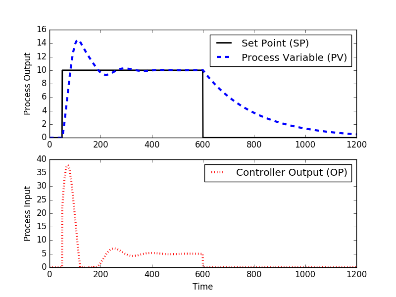
PI Control
Configure the controller to add together an integral term in addition to the proportional control with `K_c = 2`. Simulate the PI controller response with integral reset times `\tau_I=200, 100, 10`. Include a plot of the integral of the fault between the set bespeak (SP) and process variable (PV) with anti-reset windup. Explain what happens and why.
Open Loop Response with Dead Time
Add dead time `\theta_p=100` as an input delay. Simulate the behavior for making a footstep change in manual fashion from 0 to 10 (and back). Explain what happens in terms of oscillations.
P-only Command with Expressionless Time
With the dead time, simulate the response of a P-merely controller with `K_c=2` and `K_c=0.5`. Implement a ready point change from 0 to 10 and dorsum in automated mode (closed-loop). Include a plot of the error between the set bespeak (SP) and process variable (PV). What happens with increased `K_c` in terms of offset and oscillation?
PI Control with Dead Time
Simulate the response of a PI controller with `\tau_I=200`. Include a plot of the integral of the mistake betwixt the set signal (SP) and procedure variable (PV) with anti-reset windup. Explain what happens and why. Explain the results.
Summary Questions
- Based on the observations in manual mode, is the process stable or unstable?
- Why does P-but command have persistent starting time?
- What is the result of dead time on P-but and PI control?
- If the process is stable, why tin the command system make information technology unstable?
Sample Code
import numpy equally np
import matplotlib.pyplot as plt
from scipy.integrate import odeint
# specify number of steps
ns = 1200
# define fourth dimension points
t = np.linspace ( 0 ,ns,ns+i )
# mode (manual=0, automatic=1)
mode = one
grade model( object ):
# process model
Kp = 2.0
taup = 200.0
thetap = 0.0
class pid( object ):
# PID tuning
Kc = two.0
tauI = 10.0
tauD = 0
sp = [ ]
# Ascertain Gear up Point
sp = np.zeros (ns+1 )# fix point
sp[ 50:600 ] = x
sp[ 600:] = 0
pid.sp = sp
def process(y,t,u,Kp,taup):
# Kp = process gain
# taup = process time abiding
dydt = -y/taup + Kp/taup * u
return dydt
def calc_response(t,style,xm,xc):
# t = time points
# fashion (transmission=0, automated=one)
# process model
Kp = xm.Kp
taup = xm.taup
thetap = xm.thetap
# specify number of steps
ns = len (t)-1
# PID tuning
Kc = xc.Kc
tauI = xc.tauI
tauD = 90.tauD
sp = xc.sp# set indicate
delta_t = t[ 1 ]-t[ 0 ]
# storage for recording values
op = np.zeros (ns+ane )# controller output
pv = np.zeros (ns+ane )# process variable
e = np.zeros (ns+1 ) # error
ie = np.zeros (ns+1 )# integral of the error
dpv = np.zeros (ns+1 ) # derivative of the pv
P = np.zeros (ns+ane ) # proportional
I = np.zeros (ns+one ) # integral
D = np.zeros (ns+i ) # derivative
# step input for manual control
if mode== 0:
op[ 100:] = 2
# Upper and Lower limits on OP
op_hi = 100.0
op_lo = 0.0
# Simulate time delay
ndelay = int (np.ceil (thetap / delta_t) )
# loop through fourth dimension steps
for i in range ( 0 ,ns):
e[i] = sp[i] - pv[i]
if i >= 1:# calculate starting on second cycle
dpv[i] = (pv[i]-pv[i-1 ] )/delta_t
ie[i] = ie[i-one ] + e[i] * delta_t
P[i] = Kc * due east[i]
I[i] = Kc/tauI * ie[i]
D[i] = - Kc * tauD * dpv[i]
if way== 1:
op[i] = op[ 0 ] + P[i] + I[i] + D[i]
if op[i] > op_hi:# check upper limit
op[i] = op_hi
ie[i] = ie[i] - e[i] * delta_t # anti-reset windup
if op[i] < op_lo:# bank check lower limit
op[i] = op_lo
ie[i] = ie[i] - e[i] * delta_t # anti-reset windup
# implement fourth dimension delay
iop = max ( 0 ,i-ndelay)
y = odeint(process,pv[i] , [ 0 ,delta_t] ,args= (op[iop] ,Kp,taup) )
pv[i+1 ] = y[-1 ]
op[ns] = op[ns-1 ]
ie[ns] = ie[ns-1 ]
P[ns] = P[ns-1 ]
I[ns] = I[ns-1 ]
D[ns] = D[ns-1 ]
render (pv,op)
def plot_response(north,mode,t,pv,op,sp):
# plot results
plt.effigy (n)
plt.subplot ( ii , ane , 1 )
if (mode== i ):
plt.plot (t,sp, 'k-' ,linewidth= 2 ,characterization= 'Prepare Point (SP)' )
plt.plot (t,pv, 'b--' ,linewidth= 3 ,characterization= 'Procedure Variable (PV)' )
plt.legend (loc= 'best' )
plt.ylabel ( 'Process Output' )
plt.subplot ( 2 , 1 , two )
plt.plot (t,op, 'r:' ,linewidth= 3 ,label= 'Controller Output (OP)' )
plt.fable (loc= 'best' )
plt.ylabel ( 'Process Input' )
plt.xlabel ( 'Time' )
# calculate stride response
model.Kp = 2.0
model.taup = 200.0
model.thetap = 0.0
mode = 0
(pv,op) = calc_response(t,mode,model,pid)
plot_response( one ,fashion,t,pv,op,sp)
# PI control
pid.Kc = 2.0
pid.tauI = 10.0
pid.tauD = 0.0
mode = 1
(pv,op) = calc_response(t,way,model,pid)
plot_response( 2 ,mode,t,pv,op,sp)
plt.show ( )
Assignment
Come across Velocity PI Command
Source: https://apmonitor.com/pdc/index.php/Main/ProportionalIntegralControl
0 Response to "Pi Controller Phase Rises Again Before Falling"
Post a Comment